Exploratory data analysis (EDA) isn’t just for data scientists. Anyone that uses a system that emits data can benefit from the tools of EDA. And since charity begins at home, what better way to motivate this than a short post using DataHaskell tools to analyse GHC profiling logs.

By treating performance analysis as a data exploration problem, we may unlock insights that might be difficult to see in a static report.

This article is for you if:

• • You’ve profiled Haskell programs before and want a more flexible way to explore the data beyond what static tools provide: filtering, joining, and comparing runs programmatically.
• • You’re comfortable with data tools (pandas, R, SQL) but haven’t worked with GHC’s profiling infrastructure this will show you how to bridge that gap.
• • You want to compare performance across code changes by diffing two profiling runs to see exactly what got better or worse, attributed to specific cost centres.
• • Or you’re just curious about DataHaskell!

The example program

For our scenario today we’re going to compare the memory behaviour of two variants of a simple summing function. The first is a textbook strict fold:

sumFast :: B.ByteString -> Int  
sumFast bs =  
  let xs = parseAll bs  
   in foldlStrict (\ !acc x -> acc + x) 0 xs

The second version is almost identical, but it retains a sample of partial sums as it runs—a controlled memory leak that accumulates data over time:

data Acc = Acc !Int !Int !SampleList

sumLeaky :: B.ByteString -> Int  
sumLeaky bs =  
  let xs = parseAll bs  
      Acc s _ samples = foldlStrict step (Acc 0 0 Nil) xs  
   in sampleLength samples `seq` s  
  where  
    step (Acc s i history) x =  
      let !s' = s + x  
          !i' = i + 1  
          !history' = if i' `rem` 50000 == 0  
                      then Cons s' history  
                      else history  
       in Acc s' i' history'

Both compute the same result. Both have similar runtime. But one retains memory that the other doesn’t—and we want to see that difference in the profiling data.

To generate eventlogs, you need to:

1. Compile with profiling enabled: cabal build --enable-profiling --profiling-detail=all-functions -O2
2. Run with the right RTS flags: cabal run your-program -- +RTS -hc -l-agu -RTS

Here -hc requests heap profiling by cost centre (we’ll explain what that means shortly), and -l-agu enables the eventlog while disabling some less relevant event types. This produces a .eventlog file alongside your executable. For our example, we generate two: fast.eventlog and leaky.eventlog.

The standard tool for visualising these logs is eventlog2html, which produces beautiful interactive HTML reports.

It’s excellent for getting a quick overview—but sometimes you need more. You might want to filter to specific cost centres, compare two runs side-by-side, compute derived metrics, or ask questions the tool’s authors didn’t anticipate.

We’d like to see if we can get this and then more using a SQL-like API to explore our eventlog data. In this blog post we’ll do two things: firstly, we’ll show how to regenerate the heap usage chart from eventlog2html. Secondly we’ll show how to use operations like join to diff two runs.

Generating eventlogs

GHC can emit detailed runtime information into eventlog files. These binary logs contain a stream of timestamped events: garbage collection statistics, heap samples, cost centre attributions, and more.

From eventlogs to dataframes

An eventlog is just a pile of raw facts with disjointed descriptions of what happened and when it happened. To turn it into answers, we need tools that can ingest event streams, normalise timestamps, join disparate metrics, and visualise relationships.

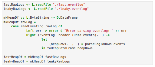
We’ll use the ghc-events library to parse the binary format, then load the data into a DataFrame. This gives us a familiar columnar interface. If you’ve used pandas or dplyr, the operations should feel natural.

We write some custom code to parse eventlog files into structures that we’ll eventually turn into dataframes.

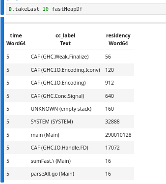
After parsing, we have a table with three columns: time, cc_label (the cost centre label), and residency (bytes retained):

A quick note on cost centres

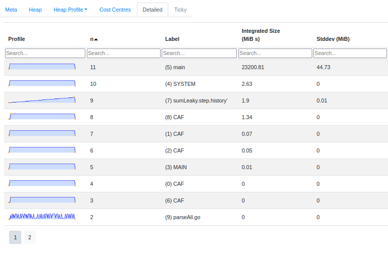
A cost centre is GHC’s unit of attribution for profiling. When you compile with -profiling-detail=all-functions, GHC inserts cost centres at function boundaries. Each heap sample then records how much memory is attributed to each cost centre. Cost centre labels look like sumLeaky.step.history' (Main). That’s the function history’ defined inside step inside sumLeaky, in the Main module. These hierarchical names let you trace allocations back to specific expressions in your code.

Aggregation

Raw performance data is noisy. The runtime might emit a “Heap Size” event every few microseconds, creating thousands of data points per second of runtime. Using DataFrame functions, we can group these by a coarser time grain and calculate the mean, effectively “smoothing” the signal.

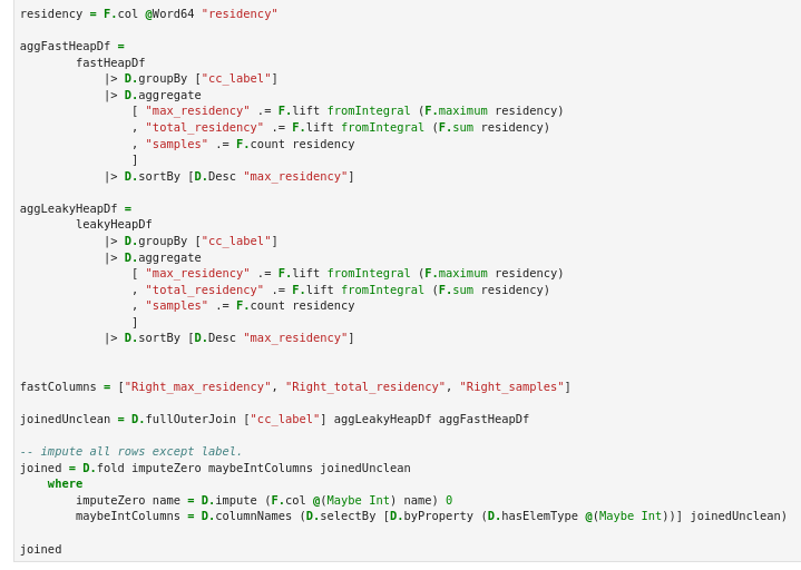
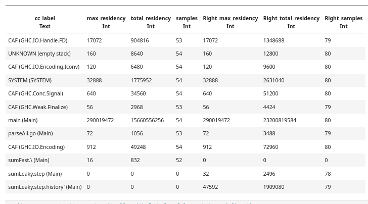
Now we have one row per cost centre, with summary statistics. But the real power comes when we compare runs.

Joining two profiling runs

To diff the fast and leaky versions, we perform a full outer join on the cost centre label:

The result tells us exactly where the memory went. The history’ binding where we cons onto the sample list accounts for the retained memory.

Correlating different metrics

Eventlogs contain multiple types of events. Beyond heap samples by cost centre, we get:

• • HeapLive: actual live bytes after GC
• • HeapSize: total heap size requested from the OS
• • BlocksSize: memory in block allocator

We can parse these into separate DataFrames, aggregate by time, and join them together:

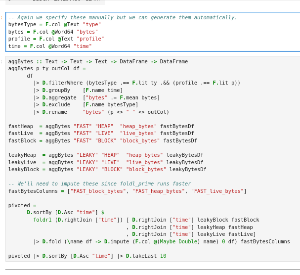
This gives us a wide table where each row is a time bucket, and columns show different metrics for each run:

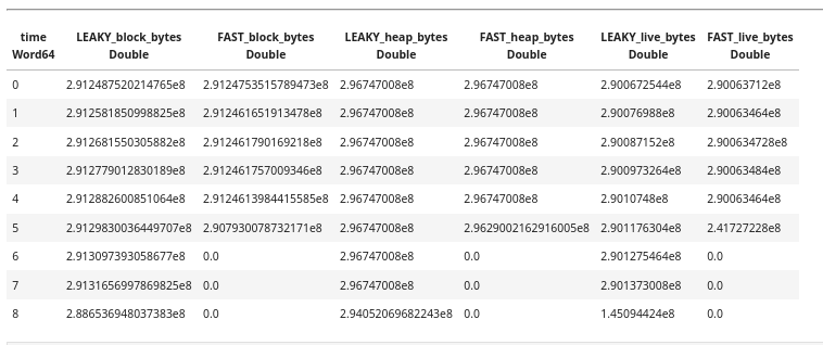
Plotting the results

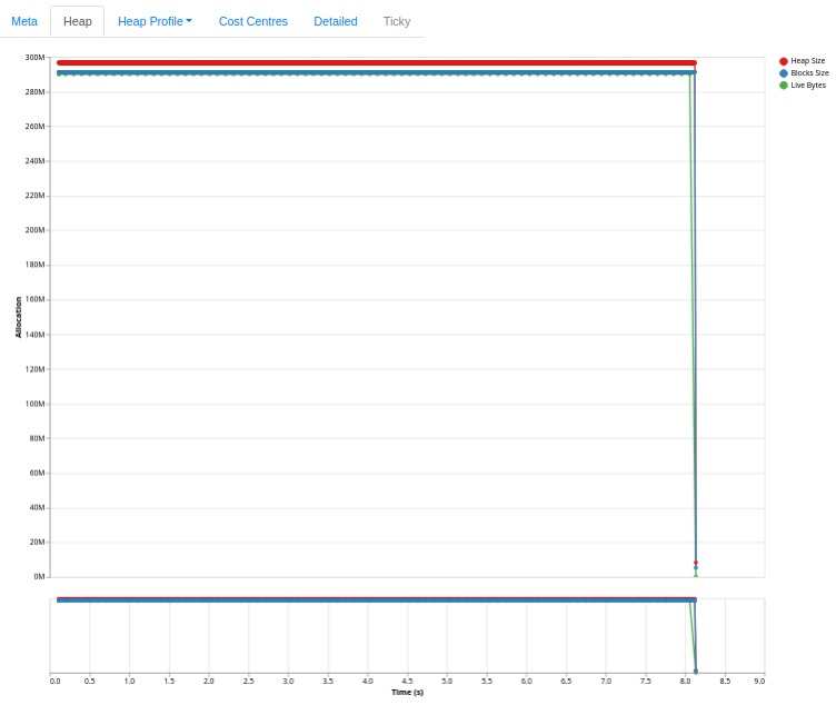
Now we can go ahead and plot the famous eventlog2html heap usage chart with both runs in the same chart.

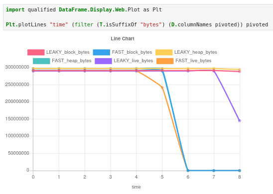
We can “zoom in” on the chart by taking the first 5 rows and see the difference in live bytes.

The leaky version shows steadily increasing live bytes; the fast version stays flat. But more importantly, we can now query this data: what’s the rate of growth? When does the leak become significant? Does block size track live bytes, or does the allocator hold onto memory after GC reclaims it?

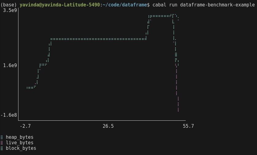
As an added bonus, We can run our profiling code in GHCi/a regular script as well and produce similar output.

What we learned

The notebook captures the entire pipeline from raw eventlog to final visualisation. Re-run it after a code change and you get an updated diff automatically. Because everything is in DataFrames, we can filter to specific time ranges, compute ratios, correlate with GC events, or export to CSV for further analysis in other tools.

This gives us a flexible way of exploring performance.

The full notebook is available to explore in the DataHaskell playground.

What’s next?

We are currently working on turning this workflow into a dedicated library. We’re working with developers to see what data and charts will be the most useful for understanding performance. Our goal is to provide a seamless bridge between the GHC RTS and high-level analysis tools. Along with the library, we will be providing guides on how to use these data-science techniques to diagnose specific performance pathologies.

As always watch this space and if this sort of work is interesting to you, hop over to the DataHaskell discord to get in on the action.

Contributors: Michael Chavinda, Jireh Tan, Tony Day, Laurent P. René de Cotret